ERP Processing Using EEProbe
Outlined by Darren
Parker 2006
Part 1: Transfer Data
Why?
EEProbe needs to be able to access your data from Tomcat in EEProbe’s preferred format.
How?
Behavioural data (behavioural data ends with extensions like *.da1 *.da2 *.da3 *.da4 *.log) is saved onto Blue (sometimes Tomcat) and the EEG data is saved onto Red (*Blue and Red are the names of the data acquisition computers). On Blue, go into C: /data/<experiment> (*whenever there are <brackets> it indicates that this is interchangeable between experiments and sometimes conditions) and see if your data has been saved here. If so, organize the subject’s data into a single folder using the naming convention for that experiment (to make a folder right click in the folder and select New -> Folder). For example, subject number six in the third item specific experiment we run is named is0306 and is found in the is03 folder. If you do not see the data on Blue, then it is likely on Tomcat already. Open up Network Places and go to data on Tomcat. Choose the corresponding experiment folder and find the behavioural files to organize them into a folder for the subject.
When a subject folder is made, it should be copied to/made in Tomcat as per the structure in figure 1. This is EEProbe’s preferred format, with data on Tomcat being the project directory, dt01 one of the experiment folders and dt0101 being one of the subject directories.
When this is done move on to Red. Go to C: /data and copy the *.bdf file from there to the subject’s folder that you have created on Tomcat. By the end you should have all of the behavioural files (*.da1 *.da2 *.da3 *.log) and the EEG file (*.bdf) in the subjects directory on Tomcat.
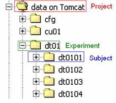
Figure 1
Steps for data transfer:
- Find all of a subject’s files, both behavioural and EEG.
- Organize all of a subject’s files into their Subject folder. Do this by creating a new folder in the Experiment folder with the subject’s number (e.g. dt0101 for subject one in the dt01 experiment).
Part 2: Importing Data
Why?
The *.bdf file format that our ActiView records in is not recognized by EEProbe. The *.bdf format has to be converted over to *.cnt format that EEProbe can recognize.
How?
This has to be done in Linux so go to a computer with Linux running or boot any of the computers into Linux by restarting. When in Linux, click on the star button in the lower left hand corner. Then click on System -> Terminals -> <any terminal>. At the prompt, type in eeprobe (case sensitive). This should bring up the EEProbe databrowser as seen in figure 2. You will see three columns at the top organized into Experiment, Subject and Datafile, with the Workset below.
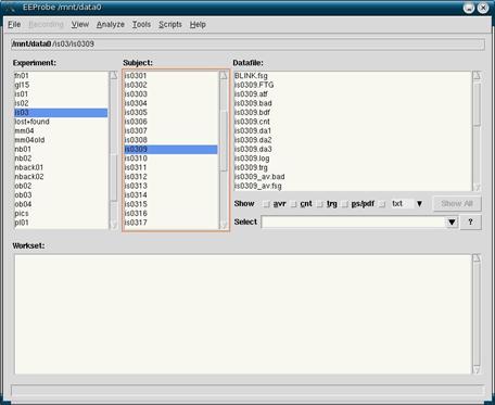
Figure 2
Start by finding the experiment and highlight it, then find the subject and highlight them. This will help set the defaults for importing. Now, Click on File in the top left corner and click on Import Data…
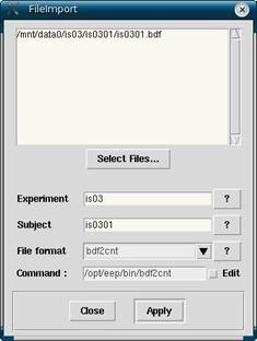
Figure 3
This will bring up a window as seen in figure 3. Make sure that the Experiment and Subject fields are correct (they should be if you selected the Experiment and Subject already in the databrowser). Also make sure that your File format converter is set to bdf2cnt (this is the default format and should not need to be changed unless you are using old data or data from other sources). Never touch or change the Command parameter since this will change automatically with File format.
Click on Select Files… to find the *.bdf to be changed over to a *.cnt file. You will have to click into the experiment and subject directories here again, and then the *.bdf will be the only file listed. When you have selected it and see it in the top window as seen in figure 3, then you are ready to click Apply. After doing so, you will see in the Workset of the databrowser your newly made *.cnt file.
Steps for importing data:
- Boot Linux
- Open a terminal (i.e. Konsole) and type in “eeprobe” (case sensitive).
- Under Experiment highlight the experiment, then under Subject highlight the subject that is having their bdf converted to cnt.
- Click on File -> Import Data
- Double check that Experiment, Subject and File format fields are correct.
- Click Select Files…and find the subject’s bdf.
- Click Apply
Part 3:
Retriggering
Why?
If you double click on your *.cnt file, you will see the relative electrical activity at all the channels, and at the bottom of the screen you will see blue numbers that indicate that a trigger has occurred at this particular time point. Each stimulus or response has its own unique trigger. There are some limits to the triggers passed on to the *.bdf file. They can only be three numbers long, and stimulus triggers do not indicate anything about the response, since the triggers are produced on the fly. To make a long story short, the triggers produced automatically are insufficient, and we retrigger to get all the extra information we need and want.
How?
There are many methods of retriggering. The following is the labs most common method of retriggering. It may change from experiment to experiment, but if you see *.da3 files present for the subject, this is almost certainly the method you will follow.
For this step Windows is required. Reboot any computer other than Tomcat or Brain and upon start up, make sure that windows is selected (default is Linux). Open Excel and open up the *.trg file and the *.da3 file from within the subject’s directory. You will be given some options to how justification is set up. You will have to make sure that delimited is selected (not fixed width) and then click Next. Make sure that tabs and spaces are both checked off, and then click on Finish.
From the *.da3 file, you are going to want to copy and paste the last 3 rows of data (you do not need to copy the headings). Paste these columns into the *.trg file and make sure that you line up the right most column of the *.trg file with the left most column of the *.da3 file. Scan through the data making sure that these columns line up throughout. If for some reason the column triggers do not match up you will want to adjust the rows pasted from the *.da3 file by cutting and pasting them to line up properly. It is critical that this is done correctly. The goal is to replace the old triggers of the *.trg file with the new triggers which are the last column of the *.da3 file. If the positions are not put in place properly, conditions can not be averaged together properly. When the rows are lined up properly you will want to delete some columns so that the old triggers are replaced altogether by the new triggers. An example of this can be seen in Figure 5. Do this by deleting the columns with the old triggers, the copy of the old triggers pasted from the *.da3 file, and the StimTime/RespTime column from the *.da3 file.
There are two additional steps to follow so that EEProbe will properly read the triggers from your trigger file. The first is to fill in any empty trigger rows with a “9”. If any of the timepoints do not have a trigger assigned to it, then any following triggers will not be read in properly. To do this, click on the top of the trigger code column (in the Figure 5 example, this is column D) in order to have it select the entire column. Click on Edit -> Replace. Leave the Find what field blank, and in the Replace with field enter 9. You will want to delete the very top 9 because the top row is the header and there are no triggers or timestamps there.
In some cases rows 2 and 3 will contain some garbage header information that looks like funny boxes. If this happens then delete these two rows so that the triggers start right away at row 2. If you do not do this EEProbe will not be able to see any triggers and the trigger file will have to be fixed until it works.
Save your trigger file by clicking on the save button and then clicking yes or save to anything that Excel asks of you. Close Excel using the same yes or save strategy. Boot into Linux and open EEProbe. Select your *.cnt file and put it into the Workset. Open it by double clicking on the file in the Workset and then check the blue triggers on the bottom of the screen. They should resemble the new triggers and not the old triggers. If the triggers look like the old triggers then you may not have saved the *.trg file properly. If no triggers appear at all, then open up your trigger file and compare it with the trigger transformation found in Figure 5 to see where you may have gone wrong.
Steps for retriggering:
- Boot into Windows and open Excel
- Open both the *.trg file and the *.da3 file, choose Delimited and click Next. Make sure that tabs and spaces are both checked off, and then click on Finish.
- Select the last three rows in the *.da3 file, copy and paste them into the *.trg file.
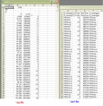
Figure 4
- Make sure that the last column of the *.trg file lines up with the first of the columns that has been copies over from the *.da3 file.
- Scan through the *.trg file making sure that the rows line up properly all the way through. Any mismatches should be corrected by adjusting columns originating from the *.da3 by cutting and pasting.
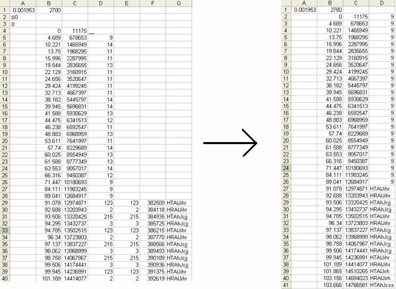
Figure 5
- When the rows line up properly, delete the columns corresponding to D, E, and F from above. The important rows to keep are the first two rows from the original trigger file, and the very last row of the da3 file.
- You may also need to delete rows 2 and 3 if they are mostly blank with only strange boxes in the first column.
- After this is done, you want to fill in the blanks in the last column. Select the entire column and then Click Edit -> Replace. Leave the find field blank, and type 9 into the replace field. Click Replace All.
- Delete the 9 in the very top row only. Save, click yes and save to everything Excel asks.
Part 4: Filtering
Why?
We are looking to reduce any extra noise in our signal as much as possible. Reducing extra noise will give us cleaner, nicer looking waveforms in the end. One of the first ways that we try to reduce noise is through filtering. Filtering in this case lets certain frequencies pass, and attempts to block other frequencies. The frequencies we are interested in which include the P1, N1, P300 etc are generally safely within 0.3 – 30 Hz. Therefore we use what is called a band pass filter that allows frequencies within that range to pass, but tries to block out frequencies that are higher or lower than those frequencies, getting rid of frequencies from electricity and lights in the room or other sources.
How?
In your EEProbe databrowser open, make sure that your *.cnt file of interest is highlighted in the Workset. Click on Analyze -> Filter Continuous to open up the filter window. You can choose to define the filter yourself by clicking on Define, or select a pre-made filter by selecting Select Filter filename.
We normally just select a pre-made filter. Click on Select which will open up a list of filters. The most commonly used filter is fs512Hz_bp0.3-30.fir.
If you want to define your own filter, click on Define and select a Highpass frequency (all frequencies higher than this frequency will pass, and lower frequencies will be blocked) and a Lowpass frequency (the opposite of highpass). You can define a filter similar to the lab’s pre-made filter by selecting a Highpass of 0.3 and a Lowpass of 30.
In either case you will want to exclude channels that do not exist or do not have any signal present. These electrodes are EXG5, EXG6, EXG7, EXG8 and Status. Do this by clicking on Except then selecting datafile and selecting the channels to exclude.
Click on Apply. When filtering is done there will be a new *.cnt file in the Workset. The name of the *.cnt file will be the same as the original, but with an “f” added to the end. For example: nb0206.cnt will create nb0206f.cnt. There will also be a corresponding *.trg file created with the added “f”. You can verify this by right clicking in the Datafile section of the Databrowser and clicking Refresh.
Steps for filtering:
- Log into Linux and open a terminal. Type in “eeprobe”.
- Click on the Experiment, then Subject, then double click on the subject’s *.cnt file putting it in the Workset, highlighted.
- Click on Analyze -> Filter Continuous.
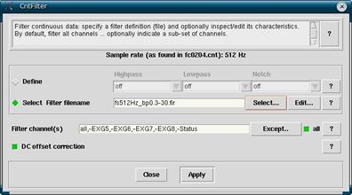
Figure 6
- Click Select. Choose a filter from the list, likely you will want fs512Hz_bp0.3-30.fir.
- Click on Except. At the top choose Datafile. Click on EXG5, EXG6, EXG7, EXG8 and Status to exclude them.
- Click Apply.
Part 5: Rejecting
Why?
While ideally subjects would never move or blink, it happens. If it happens during a trigger, and it gets included in the averaging later, it will skew the results greatly. It is necessary to reject trials with any out of the ordinary EEG behaviour to avoid adding extra noise to the averages at the end.
How?
In the Workset, make sure that your filtered *.cnt file is selected (the *.cnt file created after filtering with the “f” added to the end of the filename). Click Analyze -> Reject Continuous to open up the rejection window. Here there are a number of different settings that you likely don’t want to play around with. What you will want to do is click on Read Configuration. There are a number of rejection files depending on your needs, but you will likely want to select cntreject_allchan.cfg. This rejection file looks at all channels equally. Some of the other cntreject files only look at specific channels of interest while ignoring others.
After selecting the cntreject file you want click Apply. Pay attention to the dialogue box that comes up. In it you will see a list of the channels with a percentage next to it. The percentage is the amount of the *.cnt file rejected based on that particular channel. The lower the number the better. Some channels are more likely to have high rejection numbers than others. Because blinking causes large artifacts in the data, frontal electrodes that pick up on blinking will have higher rejection percentages than channels at the back of the head. You may want to have a cap on hand if you have any doubt about whether a channel is close to the eyes or not.
Rejection numbers can vary greatly from subject to subject. Channels that are affected by blinking are usually approximately 10% higher in their rejection statistics than other channels (this will change depending on whether they blink a lot, perhaps due to contact lenses). If channels have very high rejection statistics refer to the ERP summary sheet to see if it has already been identified as a bad channel. If it has not, then you will want to make note of it as a bad channel.
Inspect the raw data by double clicking on the filtered *.cnt file in the Workset. Skim over it to double check for any bad channels and to make sure that there are red lines at the bottom of the screen whenever the data is noisy.
Steps for rejecting:
- Make sure the filtered *.cnt file is highlighted in the Workset.
- Click on Analyze -> Reject Continuous.
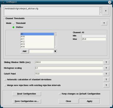
Figure 7
- Click on Read Configuration. Select cntreject_allchan.cfg.
- If you know of bad channels select them in the channel list, and hit the delete key to make your life easier later.
- Click Apply. Make note of channels with high percentage rejections. 0% is best, and some channels close to the eye may be around 10-20%. Higher than 25% on other channels is problematic and it may be a bad channel.
- Double click on the *.cnt in the Workset and inspect whether there are bad channels, and whether the rejections missed any noisy sections.
Part 6:
Rereferencing
Why?
When measuring electrical currents of any kind, a reference is required since current can’t be measure in any absolute units. For our system, the electrode CMS is essentially the reference electrode, and all the other electrodes are measured in relation to it. If we were to measure CMS itself, it would be a straight line since relative to itself, there is no difference. If you think about it, electrodes near to CMS will be producing signals from many of the same generators (the term generators refers to a cluster of cells in the brain that produce a dipole, evoking electrical current) and for this reason, the signal will be relatively small. Meanwhile, electrodes on the other side of the head will seem larger than they should be since they are picking up their own generators, as well as reflections of any of the generators that CMS is picking up.
This is corrected though rereferencing. There are a number of techniques for rereferencing. One of them is common average, where all the electrode channels are averaged together, creating a virtual reference. All of the channels subtract the virtual reference resulting in the channels being less susceptible to bias in electrode placement and location in relation to the original reference channel.
How?
In the Workset, make sure that the filtered *.cnt file is highlighted. Then, click on Analyze -> Rereference to open the rereference window. Click on Read Configuration to select a rereferencing scheme. reref1.cfg will average all the electrodes together for its newvirtual reference. Due to some noisiness in the eye electrodes, and per suggestion from the EEProbe programmers, there is another scheme rerefnoeog.cfg that does not include the eye electrodes into the newvirtual reference (but still applies the virtual reference to the channels). Therefore rerefnoeog.cfg is the configuration you will likely want to use. There is also the option to use B5 and D22 as a linked mastoid reference. The problem is that EEProbe only averages channels, while the old tools applied the Hirsch algorithm. This means that the linked mastoid reference will look funny, with electrodes at the back flatter and electrodes at the front larger. When you have decided on the rereference you want, click OK.
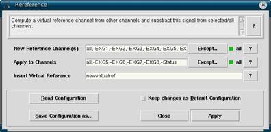
Figure 8
You will now see the electrodes that are to be used to create the new reference in the New Reference Channel(s) section, as well as the channels that the reference will be applied to in the Apply to Channels field. Notice that the subtraction symbol (-) is used to exclude channels when the “all” function is used. Particularly noisy channels that you do not want included into the new reference should be excluded as well. Please note that only extremely noisy channels should be excluded, and never more than two since it will start to skew the new reference. (Bug Alert: In version 3.2.4 of EEProbe if you type in the electrodes A1, A2, A3, B1, B2, B3, C1, C2, C3, D1, D2, D3 problems will arise. It is not worth it to exclude any of these channels as they will cause 3-10 other channels to be excluded.)
When done setting up your new reference, click Apply. When done, a new *.cnt will be produced with an “r” being added to the filename in addition to the “f” from the filtering. For example, a file that was originally named nb0204.cnt will new be nb0204fr.cnt.
Steps for rereferencing:
- Make sure your filtered *.cnt is selected in the Workset.
- Click on Analyze -> Rereference.
- Click on Read Configuration. Select rerefnoeog.cfg.
- If there are extremely noisy channels, exclude them from the New Reference Channel(s). Do this by clicking Except, then selecting Datafile, then selecting the bad channel.
- Click Apply.
Part 7: Eye Blink
Corrections
Why?
It’s important that subjects are instructed to move around as little as possible while experimental trials are occurring so that the extra noise doesn’t completely ruin any averaging. One particular form of movement that is difficult to avoid altogether is blinking. Because it is so common, various algorithms have been put together to try to remove blinks and preserve the data. While this is helpful it’s also important to remember that the tools are not exact, and if there are large numbers of blinks in the data it is still a problem.
How?
Open a new terminal so that you can use the xeog command. Before you use the command you will want to mount into the subject’s directory. Do this by typing in:
Template:
cd
/mnt/data0/<experiment>/<subject>
Example:
cd
/mnt/data0/is03/is0324
Once you are in the subject’s directory, you are ready to use the xeog command. The template of the xeog command can be displayed by typing in “xeog” and is displayed below:
Template:
xeog <cnt> <cfg> <trg in> <rej in> -a <average cfg>
Example:
xeog nb0204fr.cnt /mnt/data0/cfg/xeog.cfg nb0204fr.trg nb0204fr.rej -a /mnt/data0/cfg/cntaverage.nb02.cfg
This will open up the xeog viewer with the xcnt viewer in the background as seen in figure 9. Your focus will be on the xeog viewer, supplemented by the xcnt viewer.
The xeog viewer starts off displaying all of the Unclassified EOG events. In the raw EEG, this is everywhere that a red line is added at the bottom from when you rejected. Many of these are likely blinks, which are where the top red lines dip down, and the blue and green lines dip upward. Click the B for the best blinks that don’t appear to have any additional noise in them. You will want to classify 40 or more blinks, the more the better. You can see how many you have classified by viewing the counters at the bottom under Status. Prototypes will show you how many blinks (b) or movements (m) you have selected. You will also want to select one movement by clicking on the M. This can be any trial since we do not use movement corrections (EEProbe requires one to be selected for its calculations). When you have classified enough blinks and one movement, then click on Classification -> Calculate Propagation Factors. This will use the blinks to create an average blink (It’s more complicated than that, but that is the jist of it) to be applied to trials where a blink has occurred. When this is done go to Display -> Rejected Trials.
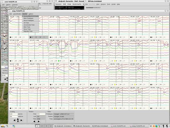
Figure 9
If it is a particularly clean subject with no bad channels and very little noisy data, you can choose to go to Classification -> Set Rejected Trials to Blink. Then click on Display -> Blink Trials. Then go through the data removing any bad trials. If a trial looks like it is clean, with no blinks, then check the raw data in the xcnt viewer. Do this by clicking on the trial in the xeog viewer, and then the xcnt viewer will automatically display the trial between the vertical black lines. Make sure that all the channels look clean before selecting it as uncorrected.
If your subject has consistently bad channels, and/or there are noisy parts in the EEG, you will probably not want to automatically set the rejected trials to blinks. You would only have to many of them back to rejected anyways. In this case go through the rejected trials manually selecting blink trials, and again, if you see a clean looking trial, double check the raw data in the xcnt, as per in the above paragraph, before designating it as an uncorrected trial.
When this is done, click on Display -> Uncorrected Trials to view the “good” data that isn’t rejected and doesn’t have any blinks. Quickly skim through to confirm that there aren’t any bad sections that have made it in, and that there aren’t any blinks that were missed. Blinks outside of the vertical black lines are okay, since only the data between the black lines is of concern.
You can see how many trials are classified as uncorrected, blinks or rejected by looking at the Trials field under Status at the bottom of the xeog viewer. A good subject will have low numbers of blinks and rejected trials and high numbers of uncorrected trials. When your trials have been correctly classified as uncorrected, blink, or rejected, you can save everything. Do so by clicking on File and saving each of Prototype Classification, Propagation Factors, Trial Classification and Trial Rejections. You can see an example in figure 10. Both Prototype Classification and Propagation Factors will be new files, so when you are saving them, at the bottom, add to the end of the filepath the file name exactly as it is in the top left corner of the xeog viewer, that is, with the “fr” at the end. Trial Classification and Trial Rejections are your *.trg file and your *.rej file respectively. Since these ones already exist, and you are simply overwriting them, you can select the file in the right hand side of the save window (make sure it is the file ending with “fr”) and then save. When you are done you can exit out of the xeog viewer.
Steps for eye blink corrections:
- Open a new terminal
- Mount into the subjects directory (e.g. cd /mnt/data0/fc03/fc0327)
- Type in the following command filling in the necessary information:
xeog
<cnt> <xeog cfg> <trg> <rej> -a <cntaverage>
For example:
xeog
fc0327fr.cnt /mnt/data0/cfg/xeog.cfg fc0327fr.trg fc0327fr.rej –a /mnt/data0/cfg/cntaverage_fc03.cfg
- Classify 40+ blinks (the more the better) and one movement.
- Click on Classification -> Calculate Propagation Factors.
- Click Display -> Rejected Trials.
- Scan through rejected trials. Classify blinks as such, and any data that looks fine can be set to uncorrected. Make sure to double check the raw data before doing this. Click on the trial of interest, then check the raw data between the horizontal black lines (you can see the raw data on the left of the screen if you click on it).
- If there are many rejected trials due to a single channel, classify them as uncorrected and make note of the channel so that it can be interpolated later.
- When done, click on Display -> Uncorrected and scan through it making sure that all the data looks good.
- This is your last chance to discern good data from bad date before averaging. Take your time to get the best results.
- Click File and save all four of Prototype Classification, Propagation Factors, Trial Classification and Trial Rejections. Do this by typing in at the end the subject’s code without forgetting to add the “fr”. E.g. fc0327fr.
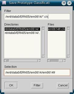
Figure 10
- Close the xeog viewer.
Part 8: Averaging
Why?
Based on individual trials, it is difficult to tease apart what parts of the signal is due to the stimulus or response of interest, and what is due to random processes occurring in the brain during the experiment. This is why we average like trials together, and why many of the experiments in the lab are highly repetitive. By averaging trials together, signal due to the stimulus or response of interest will average together because they happen every time, meanwhile other processes in the brain that are unrelated to the stimulus or response should not average together and the relatively random excess signals should cancel each other out, leaving a nice clean Event Related Potential (ERP).
How?
Go back to the EEProbe databrowser, selecting the filtered and rereferenced *.cnt file in the Workset. Click on Analyze -> Average to open up the averaging window. For this step a cntaverage file is required. This file was also required in the eye blink correction stage in order to find the various trials of interest in the EEG as well as their epoch length.
Since there should be a cntaverage file ready at this point, you can select it by clicking on Read Configuration and selecting correct one from the list. This will tell EEProbe what channels, triggers and epoch windows are required for averaging.
Make sure that EOG Compensation, and then on EOG channels are selected. If this is not done then your data will not have the blink correction applied and it will look funny with blink waves present.
When done, click on Apply. All of the averages will show up in the Workset. Right click on them and select Open to view them. Look for bad channels to be fixed in the next step, interpolation.
Steps for averaging:
- Go back to EEProbe.
- Make sure that in your Workset you have highlighted the *.cnt file you want averaged (the one with “fr” at the end).
- Click Analyze -> Average.
- Click on Read Configuration and choose the cntaverage file corresponding to your experiment.
- Make sure that EOG Compensation and on EOG channels are both selected. Click Apply.
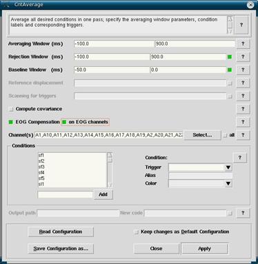
Figure 11
Part 9: Interpolating
Data
Why?
Sometimes when setting up a subject, one channel is stubborn and refuses to work properly. Other times during an experiment an electrode may come loose or problematic. Other times, for one reason or another, an electrode slips under the radar and just looks bad after averaging everything together at the end. In all of these cases you will likely want to interpolate the bad channel to avoid adding any extra noise to the grand average at the end. By interpolating a channel, EEProbe looks at the surrounding channels and calculates what the signal is most likely to be at the electrode in question.
How?
When looking at the averaged data you may notice that one electrode is extra noisy, and sticks out compared to adjacent electrodes. In such a case, you will want to make note of the bad electrode on the ERP summary sheet and then begin the steps for interpolating the bad channel.
With all of the averages highlighted in the workset, click on Tools -> Average data management -> Channel Interpolation. On this screen keep the 3D sensor position as xavr.dat (unless you are using a system differing from our current 128 channel Biosemi system). Make sure that Repair Single Channel is selected, then in Interpolate channel(s) typing in the bad electrode(s) (remember that the electrodes are case sensitive). Try to avoid interpolating large numbers of channels. If you are interpolating many channels the subject is likely not a particularly good one and the interpolation itself will be less accurate since there is less real data to work with. (Bug Alert: Channel interpolation is vulnerable to the same bug that is in the rereferencing section. Do not interpolate A1, A2, A3, B1, B2, B3, C1, C2, C3, D1, D2, D3 as of EEProbe version 3.2.5.)
Make sure that you have Output overwrites original file selected before you continue, otherwise you will end up with double the averages, and it becomes a nightmare sorting out the good *.avr files from the old ones. When done, click on Apply.
Sometimes there is only one or two noisy conditions at a particular channel that need to be interpolated. In such a case, when you select the averages to be interpolated, only select the averages that correspond to the conditions instead of all of the *.avr files. Follow all of the other steps for interpolating as above.
Check the *.avr files once more to make sure that your interpolation has helped. If the *.avr files now look good, they will be ready to be included into the grand average.
Steps for interpolating:
- Select all average files in the Workset, right click and open them.
- Ideally all channels look good and no interpolation is necessary.
- Channels that have been noted as bad, and any channels that appear irregular and noisy, should be interpolated.
- When all bad channels are noted, close the average viewer. With all average files selected click on Tools -> Average data management -> Channel Interpolation.
- In Interpolate channel(s) type in the problem electrodes. Case sensitive (use capital letters). Alternately you can select the channels by clicking on Select and Datafile.
- Make sure that Output overwrites original file is selected, and then click Apply.
- View your average files again to make sure that the interpolation helped.
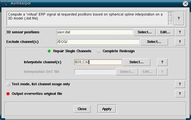
Figure 12
- Sometimes the channel may be bad for only a subset of conditions. In such a case, note the bad channel and what conditions it is bad in.
- Highlight only the conditions of concern, and then follow the instructions above from clicking on Tools -> Average data management -> Channel Interpolation onwards.
Part 10: Grand
Averaging
Why?
To gain the cleanest waves possible, you want to average together the conditions from each subject together.
How?
All of the averages from all of the subjects should be added to the workset. This can be done by right clicking on the experiment under the Experiment heading in the databrowser and then clicking on find avr -> overwrite entries in workset. This will add all the avr files to the workset. That includes unwanted averages such as previous grand averages. Make sure to clear any unwanted avr files out of the workset before grand averaging. Alternatively you can manually select the averages from each subject and add them into the workset.
When all of the desired averages are in the Workset and are highlighted, click on Analyze -> Grand Average Process. This will bring up the grand averaging window. Here you want to change all of the conditions weights from Equal to Weighted. This is done by highlighting the conditions one at a time under Grand average conditions, then under Averaging mode; change the selection from Equal to Weighted for each condition. This can be done relatively quickly by selecting the first condition, then hover the mouse over Weighted and click the left mouse button. From there just alternate between pressing the down button and the left mouse button. Depending on how quickly you do this, you may want to scan through the conditions against double checking that they have all been switched over to Weighted.
You will want to specify a new output directory in the space provided. This sets up the folder where the grand average files will be placed. You will likely want to indicate that it’s a grand average, and the date of the grand average in case there are multiple grand averages. That way we can see which is the most recent. If there are any other important characteristics they should be indicated as well. Try to keep your experiment folders as organized as possible.
If you want to avoid having to designate the conditions as weighted each time, and want to use the same output directory each time, then you will want to now click on Save Configuration as… and save a new avrprocess file with a name related to your experiment that you will remember. Next time you do a grand average, you can click Read Configuration and that will automatically apply the settings you set up previously.
Click on Apply.
Steps for grand averaging:
- Place the averages from all of your subjects into the Workset.
- With all the averages highlighted, click on Analyze -> Grand Average Process.
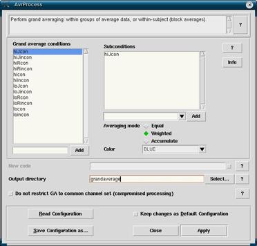
Figure 13
- First time grand averaging: highlight each condition and click Weighted instead of Equal under Averaging mode. Then type in an Output directory. Click Save Configuration as… and save your avrprocess file (must always start with avrprocess; e.g. avrprocess.is03.cfg).
- Non-first time grand averaging: Click Read Configuration and select the avrprocess file for your experiment.
- Click
Apply.